Difference between revisions of "Classifying variables in the Kepler data set"
m |
m |
||
| (5 intermediate revisions by the same user not shown) | |||
| Line 1: | Line 1: | ||
| − | ''Based on materials originally developed by Peter Plavchan ( | + | ''Based on materials originally developed by Peter Plavchan (NExScI/IPAC/Caltech) for the [http://nexsci.caltech.edu/workshop/2010/ 2010 Sagan Exoplanet Workshop]. This group project was entitled "Identifying and Classifying Variables in the Kepler Data Set."'' |
| + | |||
| + | '''NOTE: this page is still under construction''' | ||
=Introduction= | =Introduction= | ||
| Line 10: | Line 12: | ||
==Time domain astronomy== | ==Time domain astronomy== | ||
| − | |||
| − | |||
| − | |||
| − | |||
| − | |||
| − | |||
| − | |||
| − | + | All of spatially unresolved astronomy can be thought of as the exploration of a two-dimensional space: frequency and time. Astronomers have learned a lot from exploring the frequency domain, but have under-sampled the time domain in sample size, wavelength coverage, and cadence. The future of time-domain astronomy is bountiful: LSST, Pan-STARRS, Kepler, CoRoT, YSOVAR, radial velocities, ASTrO/TESS/PLATO, etc. | |
| − | + | ''Every'' star is variable at some level. Once you have a variability time-scale, you have clues to its physical mechanism. | |
| − | The signatures of non-ideal observations in time-series data are often detectable, often un-avoidable, and always annoying. For example: | + | Astronomers trip over themselves in the time-domain, because the analysis can be tricky. The signatures of non-ideal observations in time-series data are often detectable, often un-avoidable, and always annoying. For example: |
*CoRoT unavoidably moves into Earth's shadow | *CoRoT unavoidably moves into Earth's shadow | ||
*When observing from ground-based telescopes, your object rises and sets (or at least the Sun rises), introducing 1-day period aliasing | *When observing from ground-based telescopes, your object rises and sets (or at least the Sun rises), introducing 1-day period aliasing | ||
| Line 31: | Line 26: | ||
Use: | Use: | ||
*Kepler data set | *Kepler data set | ||
| − | * | + | *NASA Exoplanet Archive standard variability statistics |
| − | * | + | *NASA Exoplanet Archive periodogram and visualization tools |
*Harvard Time-Series Center classification tool | *Harvard Time-Series Center classification tool | ||
*Or, “roll your own code” | *Or, “roll your own code” | ||
| Line 41: | Line 36: | ||
*Classify the light curves | *Classify the light curves | ||
| − | ==Questions | + | ==Questions you can address by working through this project== |
*What time-scales are seen, e.g., what physical mechanisms are of interest? Ex: eclipses, flares, rotation, asteroseismology, young stars | *What time-scales are seen, e.g., what physical mechanisms are of interest? Ex: eclipses, flares, rotation, asteroseismology, young stars | ||
*What are the amplitudes of variability? (and how to identify them) Ex: How can you tell the difference between a 0.1 mag amplitude sinusoid variable with a V= 9 and 0.01 mag photon noise, vs. a V=16 object with 0.1 mag photon amplitude noise? | *What are the amplitudes of variability? (and how to identify them) Ex: How can you tell the difference between a 0.1 mag amplitude sinusoid variable with a V= 9 and 0.01 mag photon noise, vs. a V=16 object with 0.1 mag photon amplitude noise? | ||
Latest revision as of 17:59, 13 December 2011
Based on materials originally developed by Peter Plavchan (NExScI/IPAC/Caltech) for the 2010 Sagan Exoplanet Workshop. This group project was entitled "Identifying and Classifying Variables in the Kepler Data Set."
NOTE: this page is still under construction
Contents
Introduction
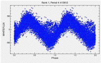
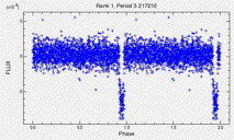
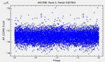
Every star has a story, told by its light curve. How do you listen to 150,000 stories at the same time? How can you (easily and accurately) tell which stories are interesting? In the figures below, one is a transit, one is noise, and one is indicative of stellar rotation, but they all have similar statistical properties. How can you tell without looking at each one by hand?
The goals for this exercise are to learn about variability statistics, periodograms, machine learning classification schemes, and the utility of ancillary information.
Time domain astronomy
All of spatially unresolved astronomy can be thought of as the exploration of a two-dimensional space: frequency and time. Astronomers have learned a lot from exploring the frequency domain, but have under-sampled the time domain in sample size, wavelength coverage, and cadence. The future of time-domain astronomy is bountiful: LSST, Pan-STARRS, Kepler, CoRoT, YSOVAR, radial velocities, ASTrO/TESS/PLATO, etc.
Every star is variable at some level. Once you have a variability time-scale, you have clues to its physical mechanism.
Astronomers trip over themselves in the time-domain, because the analysis can be tricky. The signatures of non-ideal observations in time-series data are often detectable, often un-avoidable, and always annoying. For example:
- CoRoT unavoidably moves into Earth's shadow
- When observing from ground-based telescopes, your object rises and sets (or at least the Sun rises), introducing 1-day period aliasing
- Seeing variations and blends, as well as simply a source rising (being seen through different airmasses) may introduce low-frequency noise. And, if your PSF encompasses more than one object, which one is varying? Or are they both varying?
- Systematic sources of variability can dominate and/or mask intrinsic variability in a survey. Watch out for the dreaded “red noise”! (e.g., low frequency noise)
The project
Use:
- Kepler data set
- NASA Exoplanet Archive standard variability statistics
- NASA Exoplanet Archive periodogram and visualization tools
- Harvard Time-Series Center classification tool
- Or, “roll your own code”
To:
- Define and identify a subset of ~50 interesting light curves
- Identify and handle systematics
- Identify important time-scales
- Classify the light curves
Questions you can address by working through this project
- What time-scales are seen, e.g., what physical mechanisms are of interest? Ex: eclipses, flares, rotation, asteroseismology, young stars
- What are the amplitudes of variability? (and how to identify them) Ex: How can you tell the difference between a 0.1 mag amplitude sinusoid variable with a V= 9 and 0.01 mag photon noise, vs. a V=16 object with 0.1 mag photon amplitude noise?
- How can you handle multi-periodic signals?
- How to identify, flag and remove systematic sources of variability?
- What algorithms do you use?
- How do you get and prepare the data?
- How can you use ancillary diagnostics to classify an object:
- Colors? (e.g. red = M star, giant or dwarf?)
- Phased light curve shapes ? (e.g. phased Fourier decomposition)
- How do you scale these methods to large/multiple data sets?


