Difference between revisions of "Gutermuth color selection"
m |
|||
| (5 intermediate revisions by the same user not shown) | |||
| Line 47: | Line 47: | ||
=Complicated equations can spell out simple things= | =Complicated equations can spell out simple things= | ||
| − | See [http://www.npr.org/blogs/krulwich/2012/01/10/144991340/don-t-make-me-do-this-the-equations-screamed here], and be sure to click on the complicated equations to see what they describe. | + | See [http://www.npr.org/blogs/krulwich/2012/01/10/144991340/don-t-make-me-do-this-the-equations-screamed here], and be sure to click on the complicated equations to see what they describe. Or, perhaps try googling "sqrt(cos(x))*cos(300x)+sqrt(abs(x))-0.7)*(4-x*x)^0.01, sqrt(6-x^2), -sqrt(6-x^2) from -4.5 to 4.5" (without the quotes around it). The Gutermuth (or for that matter, Koenig) method has similar complicated sets of equations, but they are just describing line segments in various color-color and color-magnitude spaces. Sit down and work through a few, even with a pencil and paper if you don't want to use Excel. You'll see, it's not so bad; it just ''looks'' bad. |
=The Gutermuth method, broken down= | =The Gutermuth method, broken down= | ||
| − | See [[media:gutermuth-appa.pdf| Gutermuth et al. 2009, Appendix A]] for the absolutely complete discussion, justification, etc. Technically, we should deredden the photometry for some of these steps, but we don’t have enough information to | + | See [[media:gutermuth-appa.pdf| Gutermuth et al. 2009, Appendix A]] for the absolutely complete discussion, justification, etc. Technically, we should deredden the photometry for some of these steps, but we often don’t have enough information to do that, and it should not matter too much for the stars we are working with. |
[[media:gutersumm.pdf|Summary of the color steps (pdf)]] | [[media:gutersumm.pdf|Summary of the color steps (pdf)]] | ||
| Line 58: | Line 58: | ||
=The Koenig method, broken down= | =The Koenig method, broken down= | ||
| − | + | ||
| + | The Koenig method is the same idea as Gutermuth, but for different bands. [[file:koenigapp.pdf|Koenig et al. 2012 appendix]] - sorry, but to get this file onto the wiki server, i had to decrease its resolution almost to illegibility. if you want a full-res copy of the file, go get the original article (Koenig et al. 2012 ApJ, 744, 130) or let me know and I'll email it to you. | ||
| + | |||
| + | =Real life situation= | ||
| + | [[Taurus catalog]] has a catalog of legitimate young stars. Where do these objects fall with respect to either the Gutermuth or Koenig colors? Which ones would be retrieved or lost by these color selections? | ||
Latest revision as of 20:14, 20 April 2015
Contents
Introduction
Spitzer is so sensitive that with just a few seconds of integration, you can easily see background galaxies. WISE is pretty sensitive too (not as incredible as Spitzer, but still often really good). Many of those background galaxies are forming stars, so they have similar colors to individual young stars. Because Spitzer's spatial resolution is not very high -- and WISE's is worse -- some of the things that Spitzer or WISE see as point sources are actually knots of ISM or resolved galaxies when viewed at higher spatial resolution. We need a good automatic way of weeding out the obvious contaminants to create a short list of sources that might actually be young stars.
No color cuts can perform this task flawlessly, though many have been discussed in the literature in the context of Spitzer observations (e.g., Allen et al. 2004, Padgett et al. 2008b, Rebull et al. 2007, Harvey et al. 2007, Gutermuth et al. 2008, 2009, Rebull et al. 2010, 2011) and now WISE too (Koenig et al. 2011).
Right after Spitzer started, there were some simple color cuts implemented to try and find these objects. There are some examples on the Color-Magnitude and Color-Color plots page. These are simple to explain and implement and visualize. However, by 2008-2009, the community had started to recognize that this was actually a more complex problem, requiring cuts in more than one space at a time. The basic approach of Gutermuth et al. (see Gutermuth et al. 2009, Appendix A) is the easiest way to impose a series of cuts in several different color-color and color-magnitude spaces all at once (by computer) to get a first guess at a list of young stars. Koenig et al. (2011) extended this method to the WISE bands. Here we now discuss this concept and these cuts in more detail.
Example of this concept using more familiar things
Sometimes, it is hard to understand what is going on during this process when you think about abstract things like distant stars or infrared colors. Let's try this with more familiar objects.
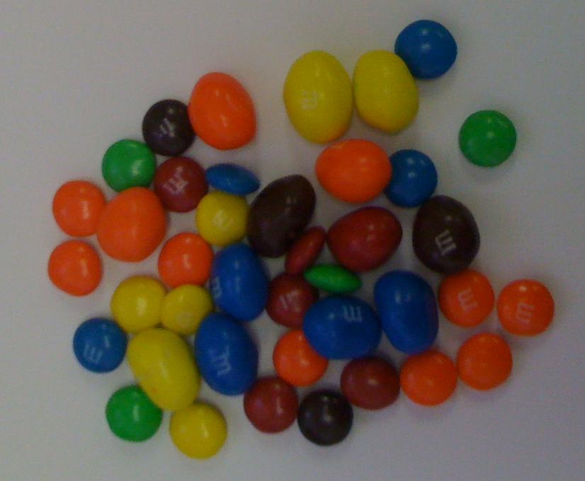
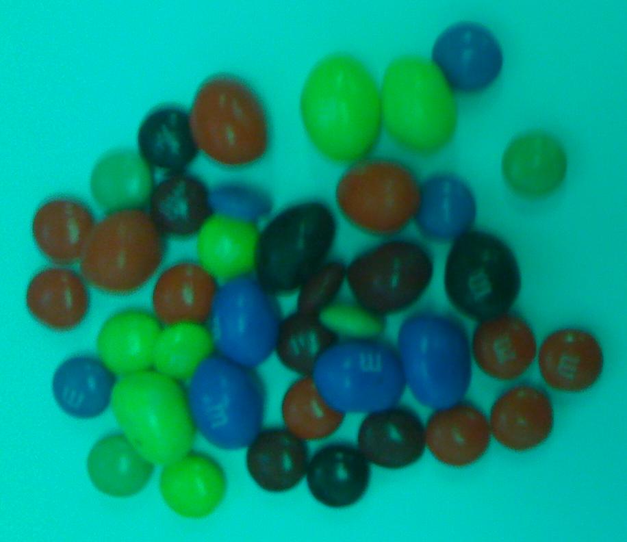
Find me the blue peanut M&Ms here:
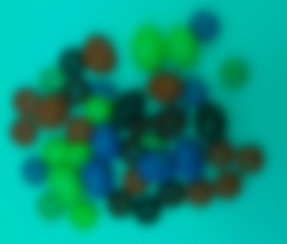
How are you going to do this? You can’t touch (or taste) them; they're too far away. Could you use their (apparent) size? But what if your camera isn’t high enough spatial resolution?
And what if one of the peanut ones has a small peanut, or is edge-on (to be compared with a face-on plain one)?
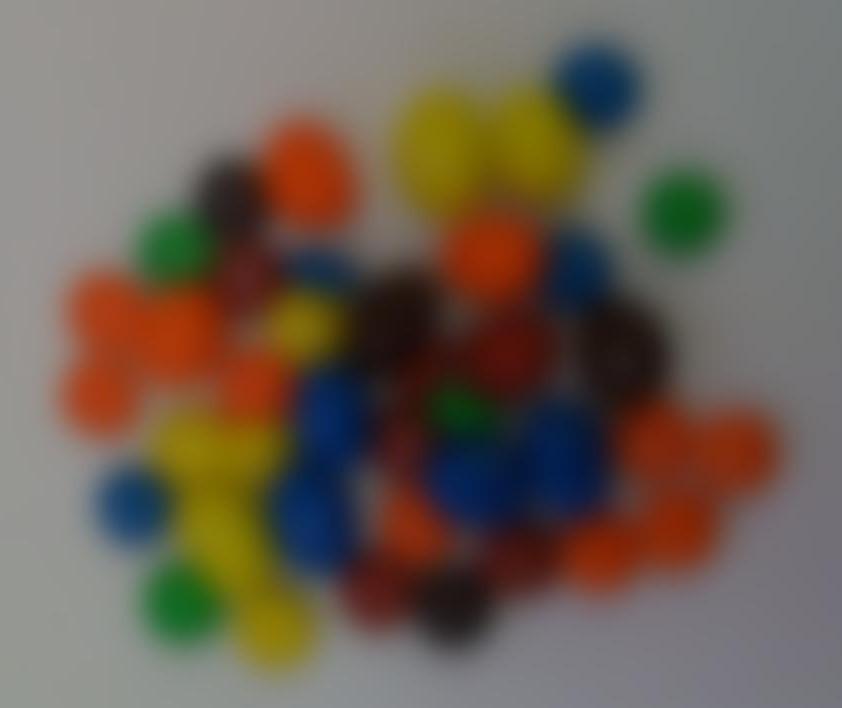
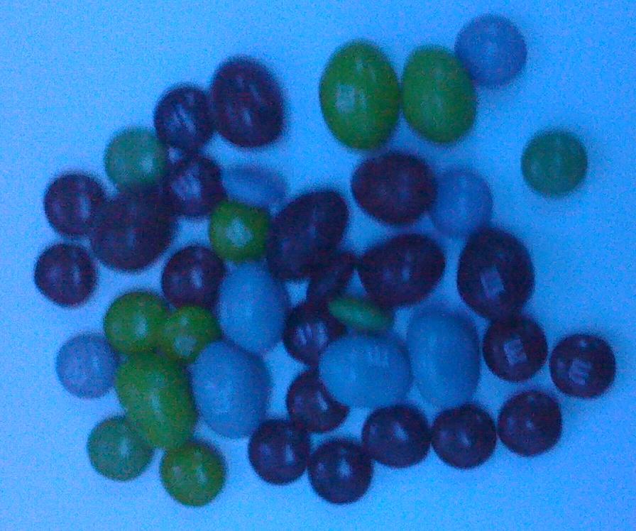
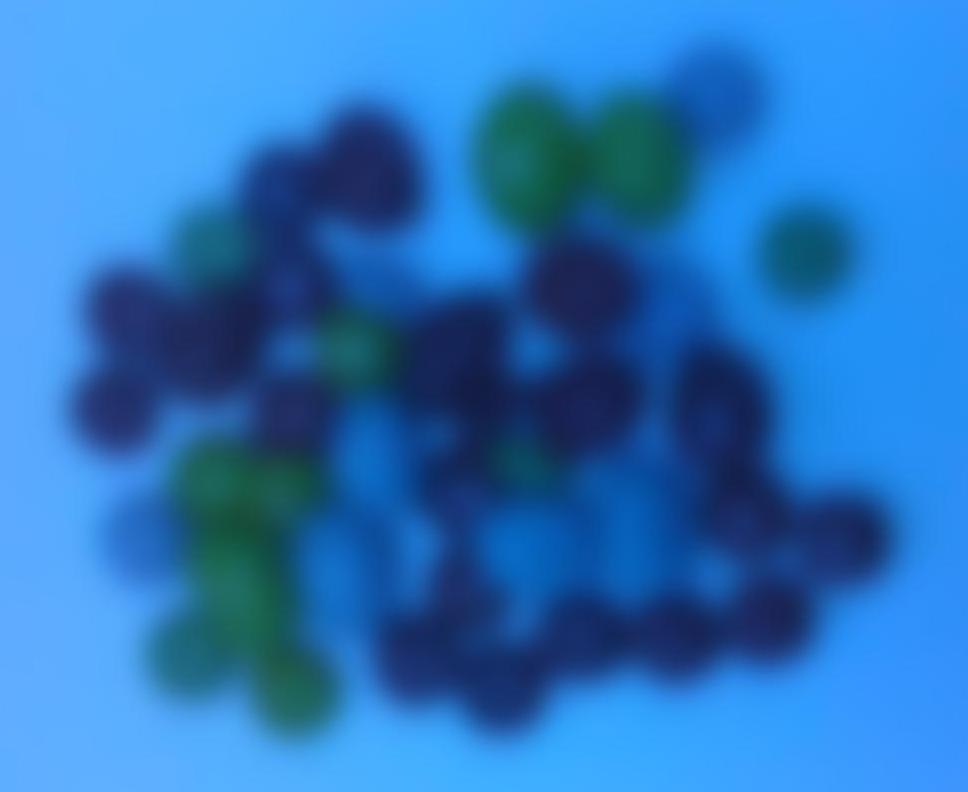
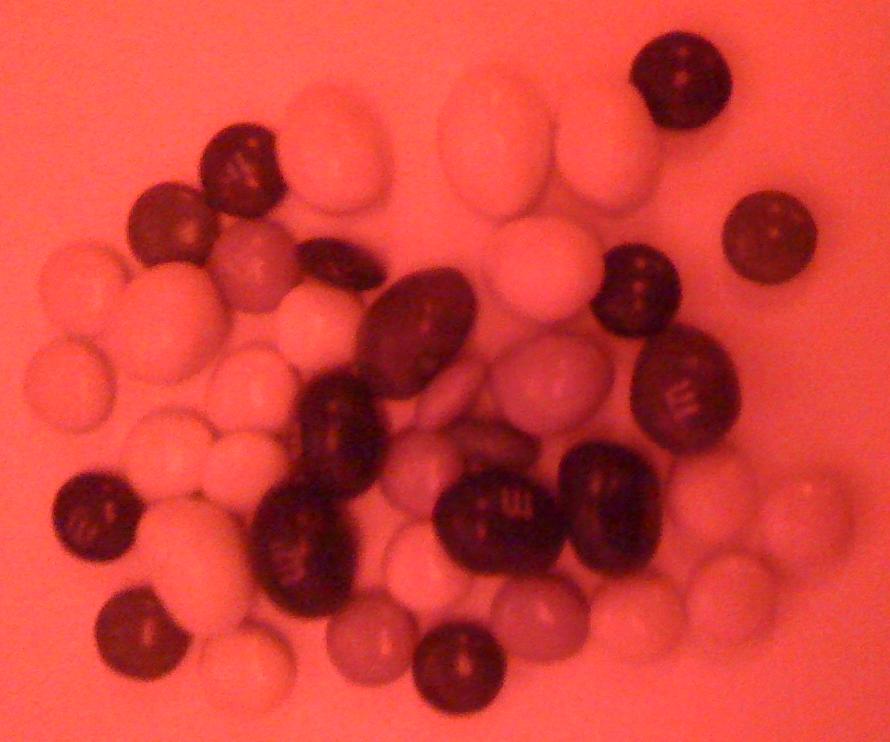
You could use their colors. Look at these various views of this same pile of M&Ms (below). Notice how the different colors of M&Ms look different in the different color filters. Remember that your camera really sees the blurry view.
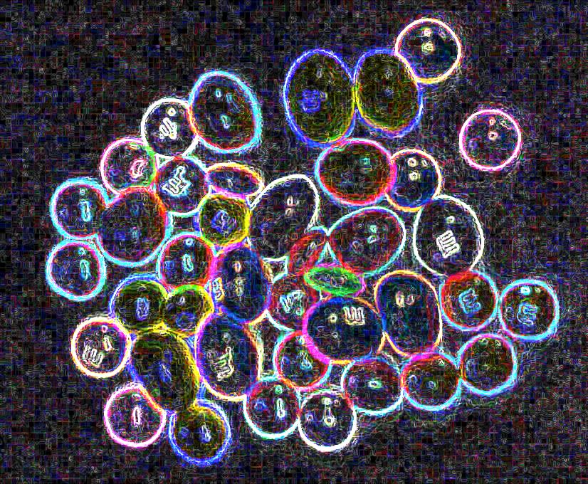
Now, maybe, you have a way of picking out the blue ones. How are you going to find the peanut ones? Remember, object size is not enough (and NASA won’t give you enough money to build a better/bigger camera). You need to find a "peanut wavelength" that can see inside the object. Here is a simulated peanut wavelength image:
For each object in the field of view, you have an estimated brightness in each of the four colors (blue, red, green, and "peanut"). You can compare the relative brightnesses in each combination. How many combinations are there? (I get six...)
- Red and green
- Red and blue
- Red and peanut
- Green and blue
- Green and peanut
- Blue and peanut
Now... For each combination, can compare colors for each object (e.g., make a plot). For each object, note properties of that object in that comparison. Then, have a big table, one entry per object, with properties of each object in each combination. You can then make an educated guess, based on properties in all available bands, which are the blue peanut M&Ms.
This is what we need to do using Spitzer or WISE colors for the young star candidates. We measure the properties of each object in all available bands. We make plots and compare them in many different color-color spaces. (You can do this manually, or let the computer do the comparison.) We make educated guesses as to which objects were likely YSOs or contaminants in each space, keeping track of which objects were which and which had which properties. (For your own sanity, this bookkeeping should all be done within the computer.)
Complicated equations can spell out simple things
See here, and be sure to click on the complicated equations to see what they describe. Or, perhaps try googling "sqrt(cos(x))*cos(300x)+sqrt(abs(x))-0.7)*(4-x*x)^0.01, sqrt(6-x^2), -sqrt(6-x^2) from -4.5 to 4.5" (without the quotes around it). The Gutermuth (or for that matter, Koenig) method has similar complicated sets of equations, but they are just describing line segments in various color-color and color-magnitude spaces. Sit down and work through a few, even with a pencil and paper if you don't want to use Excel. You'll see, it's not so bad; it just looks bad.
The Gutermuth method, broken down
See Gutermuth et al. 2009, Appendix A for the absolutely complete discussion, justification, etc. Technically, we should deredden the photometry for some of these steps, but we often don’t have enough information to do that, and it should not matter too much for the stars we are working with.
Summary of the color steps (pdf)
We can easily do the Gutermuth method up to slide 26. This provides an IRAC-based selection. We cannot deredden (we don’t have enough information), so we can’t do his JHK steps. We need to look for things that are MIPS-only; for CG4/SA101, they just fell out of the IRAC selection. We then take that initial, automatic cut and produce a short list of objects. Then we need to look at each and every one of those objects in the Spitzer bands and any other bands we can find. We then can drop computer glitches of one sort or another (duplicate sources), and we can identify any sources that are actually resolved background galaxies. Then we need to construct and examine the SED for each one, and assess them all individually for quality (like Gutermuth does too).
The Koenig method, broken down
The Koenig method is the same idea as Gutermuth, but for different bands. File:Koenigapp.pdf - sorry, but to get this file onto the wiki server, i had to decrease its resolution almost to illegibility. if you want a full-res copy of the file, go get the original article (Koenig et al. 2012 ApJ, 744, 130) or let me know and I'll email it to you.
Real life situation
Taurus catalog has a catalog of legitimate young stars. Where do these objects fall with respect to either the Gutermuth or Koenig colors? Which ones would be retrieved or lost by these color selections?
